
PATCH ANTENNAS / SUBSTRATE AND GROUND
PCB patch antenna design starts with the substrate, the ground plane and the installed geometry—not just a copper rectangle. Define the operating band, polarization, available board outline and radiation requirements first. Then calculate a starting patch, model its actual feed and finite ground, and validate the assembled product. A useful initial dimension is not a finished antenna.
This guide develops an original 10 GHz rectangular-patch example and a controlled ground-plane comparison. The dimensions are calculated teaching values. No electromagnetic simulation, prototype measurement, usable bandwidth or antenna gain is claimed for this example.
1. Specify the antenna boundary before drawing copper
Write down the lower and upper operating frequencies separately from the nominal center frequency. Add required polarization, angular coverage, installed orientation, and the minimum acceptable realized gain or efficiency under defined test conditions. An input-match target alone cannot describe coverage. For circular polarization, include an axial-ratio requirement and its angular and frequency limits; the simple rectangular example below does not establish circular polarization.
Freeze a mechanical envelope containing the board, battery, shields, fasteners, connector, cables and enclosure. Give the antenna engineer a revision-controlled drawing with material and spacing information. Identify which dimensions are fixed by the product and which can change during tuning. This prevents a successful open-board prototype from becoming the wrong reference for an enclosed product.
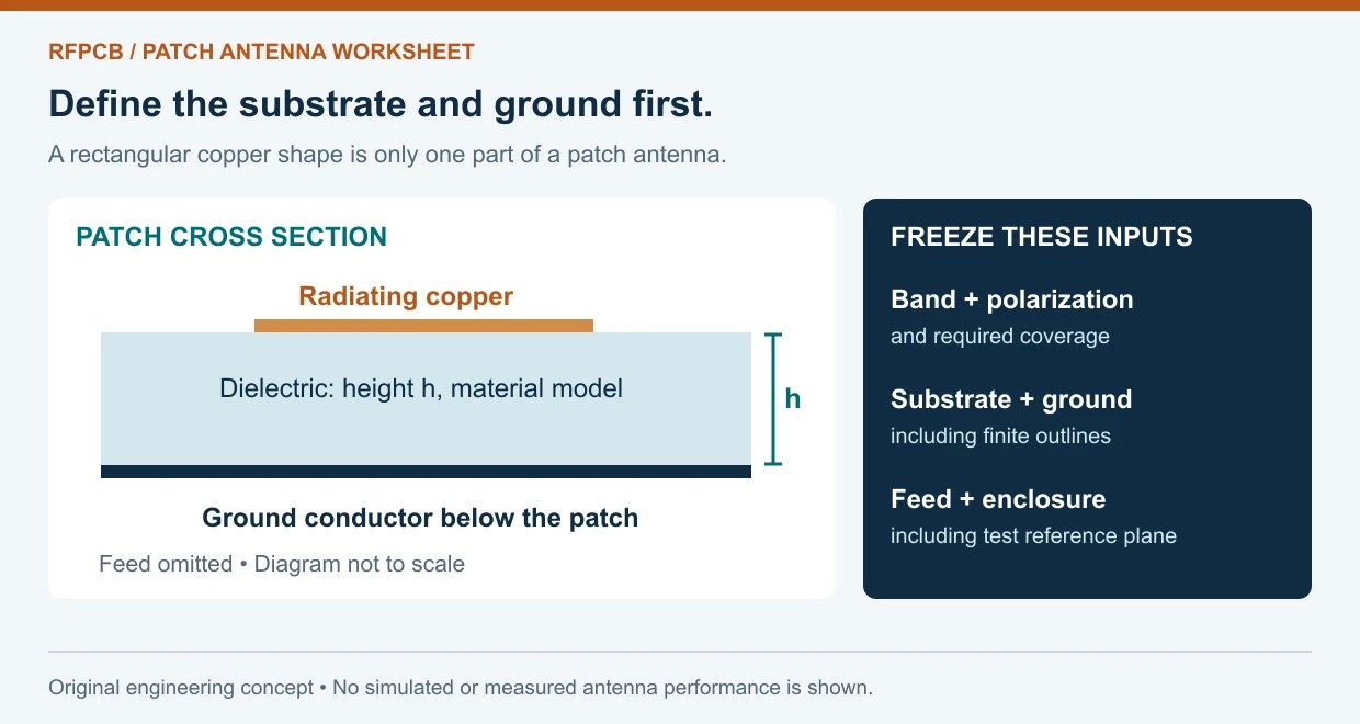
A conventional microstrip patch uses a radiating conductor above a ground plane, separated by dielectric. Keep that topology distinct from printed monopoles or antenna modules with manufacturer-defined copper keepouts. A generic instruction to remove all copper below every PCB antenna would change the patch into a different structure. Likewise, adding shorting vias through its radiator requires deliberate redesign.
2. Record the substrate model, not only its trade name
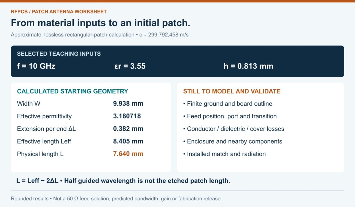
For this example, select a nominal dielectric height h = 0.813 mm and scalar relative permittivity εr = 3.55 at a 10 GHz design frequency. These are starting inputs associated with RO4003C, not a recommendation that it is best for every antenna. The Rogers RO4000 data sheet, PUB# 92-004, revision 080322, lists a design Dk of 3.55 using the differential phase-length method over 8–40 GHz. It separately lists process Dk 3.38 ± 0.05 at 10 GHz and 23°C using clamped stripline.
Those numbers have different purposes and test methods. The process tolerance must not be attached to the design value as though the sheet specified 3.55 ± 0.05. The catalog includes 0.032 inch, approximately 0.813 mm, material; confirm the ordered construction and tolerances with the fabricator. The RO4003C manufacturing overview provides the related material-review path.
Record dielectric height between patch and ground separately from total finished board thickness. Add copper thickness, foil, finish, solder-mask coverage and any adhesive or cover layer to the model specification. The calculation below treats the dielectric as homogeneous and isotropic and neglects metal thickness and losses. A scalar design Dk is not a complete dispersive or anisotropic material model.
3. Calculate a rectangular-patch starting geometry
Use c = 299,792,458 m/s, f = 10 × 109 Hz, h = 0.000813 m and εr = 3.55. The following common thin-substrate approximations are also documented in the dimension-calculation section of the MathWorks patch-array example, R2026b. Here they are applied to a single rectangular starting patch; that source’s subsequent square-array construction is not being reproduced.
W = c / [2f √((εr + 1)/2)]
εeff = (εr + 1)/2 + [(εr − 1)/2] / √(1 + 12h/W)
ΔL = 0.412h × [(εeff + 0.3)(W/h + 0.264)] / [(εeff − 0.258)(W/h + 0.8)]
Leff = c / (2f √εeff); L = Leff − 2ΔL
W is patch width; L is its resonant length; εeff is the approximate effective permittivity; and ΔL represents the fringing extension at each radiating end. Use consistent units throughout, then convert lengths to millimeters. The calculated free-space wavelength is 29.979 mm, so h/λ0 is about 0.0271.
| Quantity | Calculated value | Meaning |
|---|---|---|
| W | 9.938 mm | Initial rectangular width |
| εeff | 3.180718 | Approximate field-dependent permittivity |
| ΔL | 0.382 mm | Extension at each end |
| Leff | 8.405 mm | Approximate half guided wavelength |
| L | 7.640 mm | Physical starting length after fringing correction |
The physical patch is shorter than Leff because this approximation accounts for end fringing. Neither number specifies a 50 Ω feed location. The equations omit finite-ground effects, the connector transition, enclosure loading, conductor losses and detailed fabrication geometry. Retain extra digits in the calculation file, but do not confuse numerical precision with manufacturing accuracy.
Check the electrical scale: use the antenna electrical-scale explorer with 10 GHz and εeff ≈ 3.180718. Its half-guided-wavelength estimate should be about 8.405 mm. That corresponds to Leff here, not the etched length L. Keep the material’s εr and the calculated εeff in separate fields.
4. Test finite ground size without moving every variable
Choose a fixed 25 × 25 mm dielectric outline for an illustrative comparison. Keep the patch, substrate height, feed geometry, material settings and external environment unchanged. Define the patch center as x = 0, y = 0 and its resonant length along x. Change only the bottom ground conductor between these diagnostic cases:
- A: 20 × 20 mm ground, centered beneath the patch.
- B: 25 × 25 mm ground, also centered.
- C: 20 × 20 mm ground, translated +2 mm along x; keep the patch and feed fixed.
These are selected study geometries, not minimum-ground rules or approved fabrication layouts. Case C still fits within the selected dielectric outline. Confirm that the chosen feed and its ground connection remain physically valid in all three cases. If they cannot, redesign the comparison and document that dependency instead of attributing every change to ground size.
The patchMicrostrip documentation distinguishes finite dimensions from an infinite ground option. Its standard object also ties substrate dimensions to ground size. Our fixed-substrate comparison therefore requires a model representation that permits independent dielectric and copper outlines. Check those solver assumptions explicitly.

For each model, record the resonance location, input impedance, realized-gain pattern, radiation efficiency and back radiation across the required band. Compare identical frequency and angular grids. Repeat with a refined mesh until changes are small enough for the project’s decision margin. An infinite-ground solution can be a diagnostic reference, but cannot validate finite board edges, mounting details or installed behavior.
5. Tune the feed while watching radiation performance
Choose and document the feed topology before optimization: probe, inset microstrip or another defined coupling arrangement. The coordinate origin, reference impedance, feed dimensions and port plane belong in the model record. A line designed for 50 Ω does not guarantee that the point where it joins the patch presents 50 Ω. Sweep feed position and patch length separately at first so their effects remain interpretable.
Set acceptance limits before comparing curves. For a one-port antenna at a defined reference plane, S11 = −10 dB means 10% of incident power is reflected and 90% is accepted. If radiation efficiency were 50%, total efficiency including mismatch would be 0.9 × 0.5 = 45%. These are illustrative power ratios, not results for the example patch. The MathWorks field-parameter definitions distinguish directivity, gain and realized gain, with realized gain including the mismatch factor 1 − |S11|².
Use a calibrated measurement reference plane and record any feed-line or fixture de-embedding. Measure the installed configuration with the intended enclosure and cable arrangement. Keep impedance evidence separate from radiation-pattern and efficiency evidence. A deeper S11 minimum can coexist with unwanted loss or an unsuitable pattern; it is not sufficient reason to release a design.
6. Turn the model into a manufacturing handoff
Release the final drawing only after the geometry and acceptance criteria have an owner. Use the material construction qualification worksheet to connect the model inputs with an orderable stackup. A substitution that preserves nominal Dk but changes thickness, foil or a cover layer still needs an engineering review.
- Construction: identify exact laminate grade, dielectric height, copper and finish, mask openings, and controlled tolerances.
- Critical artwork: dimension patch length and width, feed position, ground outline, cutouts and mechanical registration from stated datums.
- Change control: mark RF geometry that requires approval before CAM changes, substitution or repair; preserve model and artwork revision links.
- Evidence: distinguish bare-board inspection, assembled input-match testing and installed radiation acceptance, with method and conditions for each.
Archive raw measurement files alongside calibration details, photographs of the test configuration and the tested board revision. If the prototype needs tuning, update the simulation inputs and released drawings together. A handwritten trim note on one sample is not a controlled production geometry. Preserve both the original expectation and the measured difference so the next revision has an explainable starting point.
Make tolerance decisions from a sensitivity study, rather than copying an unrelated drawing. As a rough illustration, hold W, h, εeff and ΔL fixed and change only L by ±0.050 mm. Using f ≈ c/[2(L + 2ΔL)√εeff] gives approximately 9.941 GHz for the longer patch and 10.060 GHz for the shorter one. The selected length variation is not a claimed factory capability or a supplier tolerance. This one-variable estimate omits the coupled changes that a full tolerance study must include, but it shows why patch-length control belongs in the engineering discussion.
Discuss your antenna PCB requirements
For a material, stackup and manufacturing review, provide the frequency band, antenna type, enclosure outline, RF feed path, quantities and validation needs. Include the proposed substrate and ground geometry, critical dimensions and the unresolved assumptions. This gives the review a concrete engineering boundary before artwork release.
Technical sources reviewed 10 November 2026. Dimensions and study cases are original illustrative engineering examples; figures show concepts and calculations, not photographs or measured performance.
Put this into production
Request a material, stackup and manufacturing review for your RF PCB project.