

What Is EM Simulation Setup and Why Does It Matter?
EM simulation setup is the process of defining ports, boundary conditions, mesh density, and convergence criteria before a 3-D or 2.5-D electromagnetic solver begins computing field solutions. A correct setup determines whether your simulated S-parameters land within 1 dB of bench measurements or drift by 5 dB or more. Getting ports, boundaries, and meshing right is the single highest-leverage step in the entire simulation-to-hardware loop.
Most first-pass simulation failures trace back to setup errors, not solver bugs. A wave port drawn at the wrong reference plane, an absorbing boundary placed too close to a radiating structure, or a mesh too coarse at a via transition will each silently corrupt results. This guide walks through every setup decision in the order you face them: geometry preparation, port assignment, boundary selection, meshing strategy, convergence settings, and post-processing checks.
Step 1: Geometry Preparation
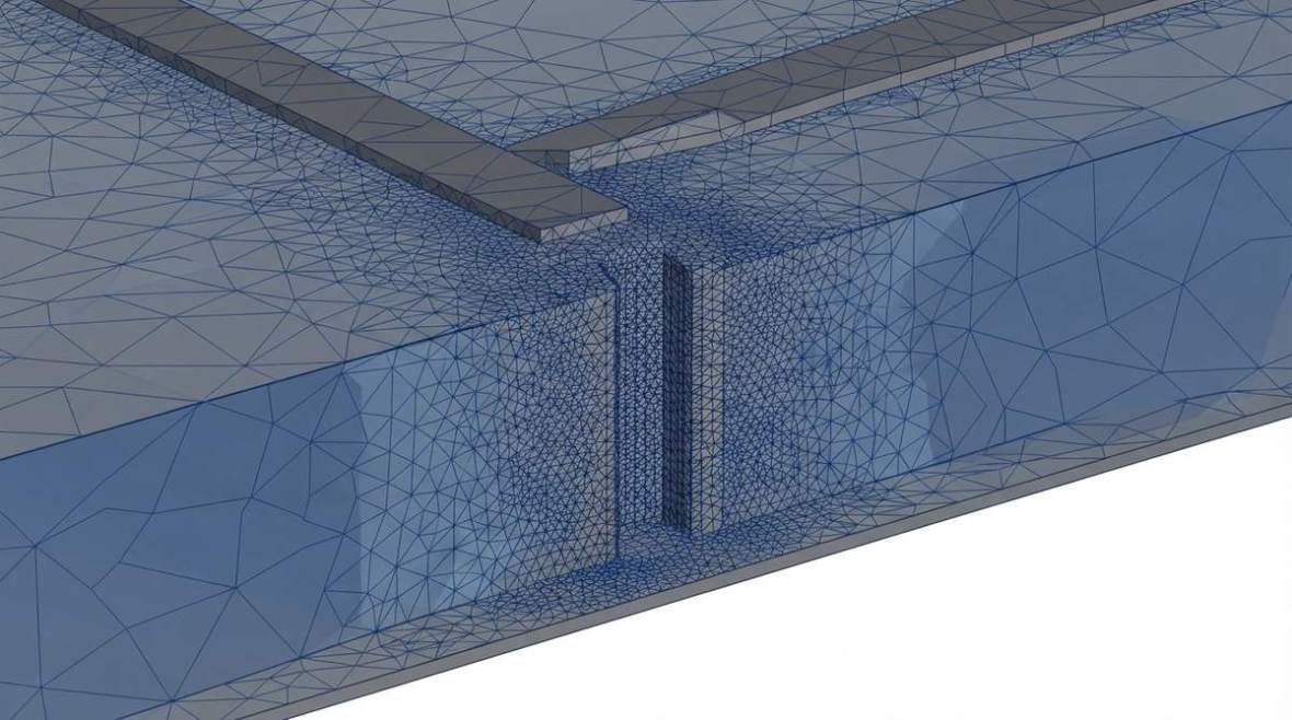
Before touching the solver, clean the 3-D model. Remove cosmetic features (silkscreen text, board outline fillets, non-functional pads) that add mesh elements without affecting field behavior. Simplify large ground planes to finite rectangles that extend at least 10× the substrate height beyond the region of interest. If you imported a layout from a tool like KiCad’s RF design workflow, verify that copper layers, via barrels, and dielectric stackup thicknesses survived the translation.
Material assignment
Assign frequency-dependent Dk and Df values, not just the datasheet 10 GHz number. Rogers RO4350B, for example, lists Dk = 3.48 ± 0.05 at 10 GHz (process method), but the design Dk used in circuit calculations is 3.66. Use the value that matches your solver’s field-solution method—full-wave solvers typically want the process Dk. Conductor losses matter above 10 GHz; model copper with surface roughness (Huray or Hammerstad–Jensen) rather than a smooth PEC sheet. The choice of high-frequency laminate directly influences how much loss the solver must capture.
Step 2: Port Assignment
Ports inject energy into the model and define the reference impedance for S-parameter extraction. Choosing the wrong port type is the most common setup mistake.
Wave ports
A wave port solves a 2-D eigenvalue problem on a cross-section to find the natural mode shape. Use wave ports when the structure has a well-defined cross-section—microstrip, stripline, coplanar waveguide, or a waveguide flange. The port rectangle must be large enough to contain the fringing fields: for microstrip, a width of roughly 10× the trace width and a height of 8–10× the substrate thickness is a safe starting point. Place the port on the outer boundary of the simulation domain so the solver does not need to mesh empty space behind it.
Lumped ports
A lumped port applies a voltage across a defined gap, much like a VNA calibration plane. Lumped ports work well for component pads, via transitions, and any location inside the model where a wave port cross-section would be ambiguous. Set the port impedance to match the system impedance (typically 50 Ω). Keep the gap physically small relative to a wavelength—under λ/20 at the highest simulation frequency—to avoid parasitic inductance from the port itself.
Floquet ports
For infinite-array antenna simulations (phased arrays, frequency-selective surfaces), Floquet ports decompose the incident field into propagating and evanescent Floquet modes. Include enough modes so that the next higher-order mode is at least 30 dB below the dominant mode at the highest frequency of interest.
Port de-embedding
If the port cannot sit exactly at the device reference plane, de-embed the excess transmission-line length inside the solver. Verify the de-embedded result by comparing the phase of S₂₁ at a known electrical length. For more advanced calibration approaches—TRL, SOLT, or 2×-Thru—see the discussion of PCB de-embedding methods.
Step 3: Boundary Conditions
Boundaries define what happens to fields at the edges of the computational domain. An incorrect boundary will either reflect energy back into the model (creating artificial resonances) or leak energy out (underestimating Q-factors).
Radiation (absorbing) boundaries
Use radiation or PML (perfectly matched layer) boundaries for any structure that radiates: antennas, open-ended transmission lines, unshielded connectors. Place the boundary at least λ/4 away from the nearest radiating element at the lowest frequency of interest. Closer placement saves memory but degrades the absorption and introduces ripple in the radiation pattern. Most solvers default to a λ/4 air buffer; for broadband sweeps (e.g., 1–40 GHz), the buffer must satisfy λ/4 at 1 GHz—75 mm of air—which can balloon the mesh. In that case, PML boundaries can be brought closer (λ/8) because they absorb over a wider angular and frequency range than first-order absorbing boundaries.
PEC and PMC symmetry planes
If the geometry and excitation share a plane of symmetry, replace that plane with a PEC (electric wall) or PMC (magnetic wall) boundary to cut the model size—and solve time—by half (one plane) or a quarter (two planes). A microstrip line running along the x-axis with a centered ground plane has an E-field symmetry that maps to a PMC plane along the propagation axis and a PEC plane perpendicular to the E-field. Applying the wrong symmetry type flips the boundary condition and kills the dominant mode; always verify by running a quarter-model and a full-model at one frequency point and comparing S₁₁.
Master/slave (periodic) boundaries
For unit-cell simulations of antenna arrays or EBG structures, link opposite faces with master/slave boundaries and apply the inter-element phase shift. Confirm the periodicity by plotting the E-field on both faces—they should be identical in magnitude and offset only by the prescribed phase.
Step 4: Meshing Strategy
The mesh discretizes the geometry into elements (tetrahedra in FEM solvers like HFSS, rectangular cells in FDTD solvers like CST). Mesh quality controls both accuracy and solve time; a 2× finer mesh can increase memory by 8× in 3-D.
Adaptive meshing (FEM)
FEM solvers refine the mesh iteratively. After each pass the solver compares S-parameters (or another convergence criterion) between successive passes. Set the convergence target to ΔS ≤ 0.01 (magnitude) with a minimum of two consecutive passes meeting the target. Allow at least 6–10 adaptive passes; if the solver converges in two passes, the initial mesh was probably already too fine and wasting time.
Manual mesh seeding
Seed finer elements in regions where fields change rapidly: trace edges, via barrels, slot apertures, and impedance transitions. A via barrel carrying a signal at 28 GHz (λ ≈ 10.7 mm in free space, shorter in dielectric) needs at least 6–8 elements around its circumference. Thin dielectric layers (25 µm / 1 mil bond plies) may need a forced minimum of 2 elements through the thickness to resolve the vertical E-field correctly.
FDTD cell size
For time-domain solvers, the maximum cell size should be ≤ λ_min / 20, where λ_min is the shortest wavelength in the highest-Dk material at the highest simulation frequency. At 77 GHz in RO3003 (Dk ≈ 3.00), λ_min ≈ 2.25 mm, so the maximum cell is about 112 µm. Copper traces as narrow as 100 µm (≈ 4 mil) then need cells at or below the trace width, which is already close to the λ/20 limit—convenient, but verify with a mesh-density sweep.
Mesh convergence check
Run the simulation at two mesh densities (for example, the final adaptive mesh and one additional refinement pass) and overlay S-parameters. If S₁₁ shifts by more than 0.5 dB or the resonant frequency of a filter or antenna shifts by more than 1%, the mesh is not converged. This single check catches more setup errors than any other.
For a deeper look at how simulated S-parameters translate into design decisions, the S-parameter fundamentals guide covers magnitude, phase, and mixed-mode conventions.
Step 5: Frequency Sweep and Solver Settings
Choose the sweep type based on the structure’s electrical behavior:
- Discrete sweep – solves independently at each frequency. Most accurate; use for narrow-band resonant structures (filters, antennas) where interpolation may miss a sharp null.
- Fast (interpolating) sweep – builds a rational-function fit from a few solved points. Excellent for broadband transmission-line models; can be 5–10× faster than discrete. Verify by overlaying a discrete sweep at a few spot frequencies.
- Transient (FDTD) – inherently broadband in a single run. Confirm that the time-domain signal has decayed to at least −30 dB of its peak before truncation, or the FFT will show ringing artifacts in S₂₁.
Set the frequency range to extend 20–30% above and below the band of interest so that band-edge behavior is captured without extrapolation.
Step 6: Post-Processing and Correlation
After solving, export Touchstone files (*.s2p, *.s4p) for circuit-level co-simulation. Before trusting the data, run these sanity checks:
- Passivity – the sum of squared S-parameter magnitudes at every port must be ≤ 1 at every frequency. A passivity violation usually means the mesh is under-resolved or ports overlap.
- Reciprocity – for passive structures, S₁₂ should equal S₂₁. Differences above 0.05 dB point to asymmetric meshing or incorrect port impedances.
- Causality – check that the impulse response is zero for t < 0. Non-causal data corrupts time-domain circuit simulations.
- Comparison to closed-form – for a simple 50 Ω microstrip, compare the simulated Dk_eff and loss per unit length to analytic models. If they disagree by more than 3%, revisit material assignments.
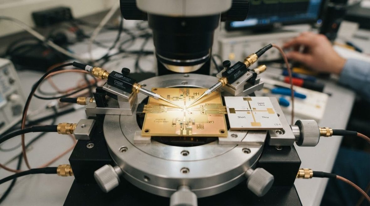
Correlation to VNA measurements is the ultimate validation. Detailed guidance on achieving agreement within 1 dB is covered in the measurement-vs-simulation correlation article.
Common Setup Mistakes and Fixes
| Mistake | Symptom | Fix |
|---|---|---|
| Wave port too small | S₁₁ baseline is −15 dB instead of < −30 dB for a matched line | Widen the port to 10× trace width, extend height to 8–10× substrate thickness |
| Radiation boundary too close | Antenna gain oscillates with frequency | Move boundary to ≥ λ/4 at lowest frequency; switch to PML |
| Wrong symmetry type | Dominant mode suppressed; S₂₁ shows deep null | Swap PEC ↔ PMC; verify with full-model spot check |
| Smooth copper (no roughness model) | Simulated loss 0.5–1.5 dB/inch lower than measured above 10 GHz | Enable Huray or Hammerstad–Jensen roughness model; use vendor’s Rz or Rrms values |
| Insufficient adaptive passes | Results change if maximum passes is increased | Allow 8–10 passes; tighten ΔS target to 0.005 for resonant structures |
EM Simulation Setup Checklist
- Clean geometry: remove non-functional features, verify stackup and via dimensions.
- Assign frequency-dependent Dk/Df and copper roughness for every layer.
- Place ports at well-defined cross-sections; size wave ports generously; keep lumped-port gaps under λ/20.
- Select boundary type: radiation/PML for open structures, symmetry planes where applicable, periodic for arrays.
- Seed mesh in high-gradient regions; set adaptive convergence to ΔS ≤ 0.01 with ≥ 2 converged passes.
- Choose sweep type; extend frequency range 20–30% beyond the band of interest.
- Run passivity, reciprocity, and causality checks on exported S-parameters.
- Correlate with a known analytic case or VNA measurement before using data downstream.
Following these steps systematically turns EM simulation from a black box into a predictable, trustworthy part of the RF PCB design cycle. For background on how simulation choices interact with radiated-emission control, the EMC design guide covers shielding, grounding, and filtering strategies that often need EM verification.
FAQ
How many mesh elements are typical for an RF PCB simulation?
A single via transition in a 6-layer board typically converges at 50 k–150 k tetrahedra in HFSS. A full connector-to-connector channel (50 mm trace, two via transitions, a connector footprint) can reach 500 k–2 M elements. Memory scales roughly linearly with element count for iterative solvers.
Can I use the same EM setup for both HFSS and CST?
The concepts (ports, boundaries, convergence) transfer directly, but the implementation differs. HFSS uses FEM with adaptive tetrahedral meshing; CST’s time-domain solver uses FDTD with hexahedral cells. Port definitions, boundary distances, and convergence criteria all need solver-specific tuning. The HFSS import-to-solve workflow details the FEM-specific steps.
What convergence target should I use for a bandpass filter?
Resonant structures need tighter convergence. Set ΔS ≤ 0.005 with at least 3 consecutive converged passes. Also run a discrete frequency sweep across the passband rather than relying solely on interpolation, because narrow rejection nulls can be missed by the rational fit.
How far should PML boundaries be from a patch antenna?
A minimum of λ/4 at the lowest simulation frequency is standard. For a 2.4 GHz patch, that is about 31 mm of air padding on each side. PML can be brought to λ/8 if memory is constrained, but validate the gain pattern against a λ/4 reference run. As documented in Ansys HFSS documentation, PML performance degrades for waves arriving at steep oblique angles, so extra padding may be needed for wide-scan arrays.
Do I need to simulate the full board or just the critical net?
Simulate only the critical structure plus enough surrounding ground and adjacent traces to capture coupling. A full-board EM simulation is rarely practical or necessary; isolating the region of interest and terminating the boundaries correctly gives faster, more interpretable results.
Ready for a quotation?
Send your requirements for a material, stackup and manufacturing review. Price and schedule are confirmed for your project.