

What Is an RF Simulation Workflow?
An RF simulation workflow is the ordered sequence of simulation, layout and verification steps that takes a high-frequency circuit from an initial schematic netlist to a physically validated PCB. It typically spans six stages: schematic-level linear/nonlinear simulation, physical layout, electromagnetic (EM) field simulation, co-simulation that stitches EM results back into the circuit, and final correlation against bench measurements. Following a disciplined workflow catches impedance mismatches, coupling and radiation effects before fabrication—problems that are invisible in a schematic-only simulation but routinely add 1–3 dB of unexpected loss or shift a filter passband by tens of megahertz.
Why a Structured Workflow Matters
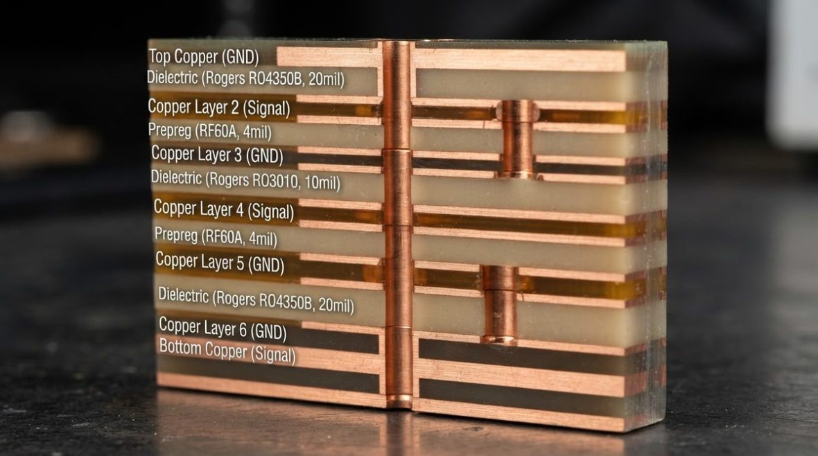
At frequencies above roughly 1 GHz, parasitic inductance, trace-to-trace coupling, via transitions and substrate dispersion all become first-order effects. A lumped-element schematic simulation models none of them. Engineers who skip EM verification and go straight to fabrication report first-pass yield rates below 50 % on tightly specified designs such as bandpass filters, power amplifier matching networks and phased-array feed networks. A structured RF simulation workflow does not eliminate iteration, but it moves the iteration into software—where each cycle takes minutes instead of the weeks required for a board respin.
Stage 1: Schematic Capture and Linear Simulation
The workflow begins with a schematic that uses vendor-supplied S-parameter models for active devices and ideal or measured models for passive components. At this stage the goal is to verify the topology: confirm gain, noise figure, stability circles and matching network Q before any layout decisions.
- Use measured S2P/S4P files from component vendors rather than SPICE models for anything above 500 MHz. A SPICE model of an MLCC capacitor, for instance, does not capture the series-resonance null that determines its useful frequency range.
- Sweep temperature and component tolerances (typically ±5 % for passives) early. If the circuit cannot meet spec across tolerance, no amount of EM accuracy will save it.
- Define clear port impedances. Most RF blocks are designed to 50 Ω, but differential pairs, balun interfaces and antenna feeds may be 100 Ω differential or an arbitrary complex impedance. Documenting the reference impedance at each port prevents confusion later.
Following RF schematic best practices at this stage—clear net naming, simulation-ready symbols, annotated port impedances—saves significant rework when the design moves into layout and EM tools.
Stage 2: Physical Layout and Stackup Definition
Once the schematic meets spec, the design moves to a PCB layout tool. Two decisions dominate RF performance: the layer stackup and the transmission-line geometry.
Stackup and Material Selection
The dielectric constant (Dk) and loss tangent (Df) of the laminate set the baseline for trace width, effective wavelength and insertion loss. A 50 Ω microstrip on RO4350B (Dk 3.48 ± 0.05, Df 0.0037 at 10 GHz) is roughly 18.6 mil (0.47 mm) wide on a 10 mil (0.25 mm) dielectric, while the same impedance on standard FR-4 (Dk ≈ 4.3, Df ≈ 0.020) is narrower and lossier. For designs above 10 GHz, consult a laminate selection guide to match Dk stability and loss to your frequency band.
Layout Rules for EM-Ready Geometry
- Keep ground-return vias within λ/20 of any transmission-line transition or connector footprint.
- Maintain reference-plane continuity under every RF trace; any slot in the ground plane becomes a slot antenna.
- Export the layout in a format your EM solver accepts—ODB++, GDSII or DXF—with metal layers, vias and dielectric definitions intact.
EDA platforms such as Altium Designer provide integrated impedance rule checks that flag violations before the layout leaves the tool. An Altium RF design workflow can automate stackup-to-solver export and reduce manual geometry cleanup.
Stage 3: EM Simulation
This is the stage where physical reality enters the model. An EM solver computes the full-wave or quasi-static electromagnetic fields on the actual copper geometry, substrate stack and via structures, then returns multi-port S-parameters that capture loss, coupling, radiation and dispersion that the schematic simulation ignored.
Choosing a Solver Type
| Solver Type | Best For | Typical Tool | Relative Speed |
|---|---|---|---|
| 2.5-D Method of Moments (MoM) | Planar structures: filters, couplers, matching networks | Keysight Momentum, Sonnet | Fast |
| 3-D FEM (Frequency Domain) | Connectors, via transitions, cavities, packages | Ansys HFSS | Moderate |
| 3-D FIT / FDTD (Time Domain) | Broadband, transient, EMC, antenna far-field | Dassault CST Studio | Moderate–Slow |
For most PCB-level RF work below 40 GHz, a 2.5-D MoM solver handles microstrip and stripline structures in minutes. An ADS Momentum workflow is a common choice for filter and matching-network verification. When the design includes vertical transitions—blind vias, press-fit connectors, ball-grid-array packages—a 3-D solver is necessary. The HFSS PCB workflow and CST Studio PCB workflow each offer detailed guidance on import, meshing and convergence for these cases.
Setting Up the Simulation Correctly
The three most common sources of EM simulation error are incorrect port definitions, insufficient mesh density and wrong material properties. A detailed EM simulation setup guide covers port types, boundary conditions and mesh convergence criteria. In summary:
- Ports: Use wave ports for transmission-line feeds and lumped ports for component pads. Mismatched port types shift the reference plane and corrupt the phase of the resulting S-parameters.
- Mesh: Converge on at least two successive adaptive passes with ΔS < 0.02 (linear magnitude). Under-meshing a coupled-line filter can hide 0.5 dB of passband ripple.
- Materials: Enter frequency-dependent Dk and Df from the laminate vendor’s datasheet at the design frequency, not the 1 MHz catalog value. Rogers RO4350B datasheet specifies Dk at 10 GHz; using the 1 GHz value introduces roughly 2 % impedance error.
Stage 4: Co-Simulation—Merging EM and Circuit
Co-simulation replaces one or more ideal schematic blocks with EM-derived S-parameter files, then re-runs the full circuit simulation. This is where the schematic world and the physical world meet.
How Co-Simulation Works
- The EM solver exports a Touchstone file (.s2p, .s4p, etc.) for the simulated structure.
- In the circuit simulator, the corresponding ideal block (e.g., an ideal coupled-line filter) is replaced with an N-port S-parameter component pointing to that Touchstone file.
- Active device models, bias networks and source/load impedances remain as circuit-level elements.
- The combined simulation runs, showing the effect of physical parasitics on system-level metrics—gain, NF, P1dB, harmonic levels.
A well-executed co-simulation typically shifts the response relative to the ideal schematic: a bandpass filter center frequency may drop 1–3 %, and insertion loss may increase 0.3–0.8 dB depending on frequency and laminate loss. These are real and expected; the point is to see them before fabrication and retune component values in the schematic while keeping the physical layout fixed, or vice versa.
Common Co-Simulation Pitfalls
- Port impedance mismatch: If the EM port was defined at 50 Ω but the circuit drives it with a complex impedance, the cascaded S-parameters are wrong. Normalize all ports to the same reference impedance, or use de-embedding techniques to remove launch structures.
- Missing parasitics: If you simulated only the filter but not the adjacent via fence or nearby trace, coupling effects are absent. Expand the EM boundary to include at least λ/4 of surrounding geometry.
- Frequency range gaps: The Touchstone file must cover the full frequency range of the circuit simulation, including harmonics for nonlinear (harmonic-balance) analysis. A file that stops at 6 GHz cannot support a 2.4 GHz PA harmonic-balance simulation that needs data to at least the fifth harmonic (12 GHz).
Stage 5: Iterate Until Convergence
Co-simulation results rarely match the original spec on the first pass. The iteration loop is:
- Identify the dominant discrepancy (center frequency shift, excess loss, poor return loss).
- Determine whether the cause is circuit-level (wrong component value, bias point) or layout-level (trace length, via placement, coupling).
- Adjust the responsible domain and re-simulate. Avoid changing both simultaneously—it obscures cause and effect.
- Repeat until the co-simulated response meets the specification with margin. A margin of at least 1 dB on insertion loss and 3 dB on return loss is prudent to cover fabrication tolerances.
Experienced designers report that two to four iterations are typical for a new filter or matching network, while a proven topology ported to a new frequency band may converge in one.
Stage 6: Measurement Correlation
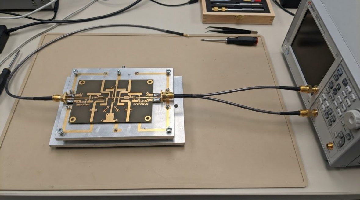
After fabrication, the prototype is measured on a vector network analyzer (VNA) and the results are overlaid on the co-simulation prediction. Discrepancies fall into predictable categories:
| Symptom | Likely Cause | Typical Magnitude |
|---|---|---|
| Uniform frequency shift | Dk different from simulation value | 1–3 % of center frequency |
| Higher insertion loss | Surface roughness, conductor loss under-modeled | 0.2–0.5 dB per inch at 10 GHz |
| Degraded return loss at one port | Connector launch or via transition not in EM model | 3–8 dB worse than simulated |
| Spurious resonance | Cavity mode in shielding enclosure or ground-plane slot | Narrow dip, 10–30 dB deep |
Closing the gap between simulation and measurement is the final, critical step. Feed the measured Dk back into the EM model, add connector models if they were omitted, and apply surface-roughness corrections (the Hammerstad, Huray or Groiss model depending on your solver). The IEEE Microwave Theory and Techniques Society publishes peer-reviewed methods for systematic sim-to-hardware correlation.
Tool-Chain Options at a Glance
| Stage | Commercial Path | Open / Low-Cost Path |
|---|---|---|
| Schematic + Linear Sim | Keysight ADS, Cadence AWR | Qucs-S, MATLAB RF Toolbox |
| Layout | Altium, Cadence Allegro | KiCad 8 |
| 2.5-D EM | Momentum, Sonnet | openEMS (FDTD, free) |
| 3-D EM | HFSS, CST Studio | openEMS, MEEP |
| Co-Simulation | ADS + Momentum, AWR + AXIEM | Qucs-S + openEMS (manual S-param link) |
Open-source tools such as openEMS can handle 3-D FDTD simulation of PCB structures with scripted geometry import, though they lack the automated co-simulation loop of commercial suites. For budget-conscious teams, a hybrid approach—KiCad for layout, openEMS for EM, and a commercial circuit simulator for co-simulation—covers most needs below 20 GHz.
Checklist: RF Simulation Workflow in Practice
- Capture schematic with measured S-parameter models; verify topology with linear/nonlinear simulation.
- Define stackup with frequency-accurate Dk/Df; lay out RF traces and transitions.
- Export layout to EM solver; set ports, boundaries and mesh; converge to ΔS < 0.02.
- Import EM Touchstone files into circuit simulator; run co-simulation.
- Iterate (adjust circuit values or layout) until spec is met with margin.
- Fabricate, measure on a calibrated VNA, and correlate; update material parameters for next design.
FAQ
When is EM simulation overkill?
Below about 500 MHz, and when trace lengths are shorter than λ/20, a well-modeled schematic simulation with parasitic extraction is usually sufficient. Above 1 GHz, or whenever traces approach λ/10, EM simulation is strongly recommended.
Can I skip co-simulation and just trust the EM result?
Only if the EM model includes every component in the signal path—including active devices, which is rarely practical. Co-simulation lets you keep accurate nonlinear device models in the circuit domain while capturing physical effects in the EM domain.
How long does a typical EM simulation take?
A 2.5-D MoM simulation of a single microstrip filter (roughly 200 mesh cells) runs in under a minute on a modern workstation. A full 3-D FEM simulation of a multilayer via transition with adaptive meshing may take 20–90 minutes depending on geometry complexity and frequency range.
What is an acceptable sim-to-measurement correlation?
For passive structures below 20 GHz, a well-correlated model matches measured insertion loss within ±0.3 dB and center frequency within ±0.5 %. At millimeter-wave frequencies (above 30 GHz), ±1 dB and ±1 % are realistic targets given fabrication tolerances and connector repeatability.
Do I need a separate EM simulation for every revision?
Only for the RF-critical structures that changed. Parameterized EM models—where trace width, length or via spacing are variables—let you re-sweep without re-importing the geometry, cutting iteration time by 50 % or more.
Ready for a quotation?
Send your requirements for a material, stackup and manufacturing review. Price and schedule are confirmed for your project.