Array Factor Calculator for Phased Arrays

What Is the Array Factor?

The array factor (AF) is the mathematical function that describes how identical antenna elements, arranged in a geometric pattern, combine their individual radiation to form a composite beam. An array factor calculator lets you plug in element count, spacing, and phase shift to instantly see the resulting beam pattern, half-power beamwidth (HPBW), and grating-lobe positions — saving hours of manual computation. The AF depends only on the number of elements, their spacing, the operating frequency, and any progressive phase shift applied across the array — not on the radiation pattern of a single element. Multiplying the array factor by the single-element pattern gives the total array radiation pattern, a principle known as pattern multiplication.

For a uniform linear array (ULA) of N isotropic elements spaced d apart along a line, the array factor is:

AF(θ) = sin(N·ψ/2) / sin(ψ/2), where ψ = k·d·sin(θ) + β

Here k = 2π/λ is the free-space wavenumber, θ is the observation angle measured from broadside, and β is the progressive inter-element phase shift used for beam steering. When β = 0 the main beam points at broadside (θ = 0°).

Interactive Array Factor Calculator

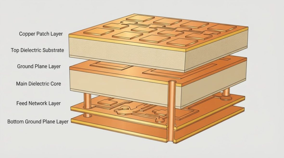
Enter your element count, spacing in wavelengths (λ), and progressive phase shift to see the normalized array factor pattern, half-power beamwidth (HPBW), and grating-lobe locations. Start with a common case: 8 elements at 0.5 λ spacing, β = 0°.

With those default values you should see a single main lobe at broadside roughly 12.8° wide (HPBW), with the first sidelobes about −13.3 dB down — the well-known result for a uniform-amplitude ULA. Increasing the element count narrows the beam; for example, doubling to 16 elements halves the beamwidth to approximately 6.4°. Widening the spacing beyond 0.5 λ will eventually push a grating lobe into visible space, which the next section explains.

Key Parameters That Shape the Array Factor

Number of Elements (N)

The half-power beamwidth of a broadside ULA scales roughly as HPBW ≈ 0.886 λ / (N·d) in radians. More elements mean a narrower beam and higher directivity — but also more feed network complexity. A 64-element array at 0.5 λ spacing yields a beamwidth near 1.6°, typical of an X-band (10 GHz) radar front end where each element sits on roughly 15 mm (≈ 590 mil) centers.

Element Spacing (d/λ)

Spacing controls both beamwidth and grating-lobe behavior. At exactly 0.5 λ, grating lobes are pushed to ±90° (the edge of visible space) and are effectively suppressed. Spacings below 0.5 λ give wider beams with no grating lobes; spacings above 0.5 λ narrow the beam but risk grating lobes entering visible space, especially when the beam is steered. For deeper guidance on maximum allowable spacing, see the grating lobe element spacing rules.

Progressive Phase Shift (β)

Applying a constant phase difference β between successive elements steers the main beam to θ₀ = arcsin(−β / (k·d)). A 90° inter-element shift on a 0.5 λ-spaced array steers the beam to 30° off broadside. Larger steering angles demand tighter element spacing to keep grating lobes out of visible space — a critical constraint in phased array antenna design.

Grating Lobes: When They Appear and Why They Matter

A grating lobe is a secondary main beam with the same peak amplitude as the desired main lobe. It appears whenever the path-length difference between adjacent elements equals a full wavelength for some angle in visible space (−90° to +90°). The condition is:

d/λ ≥ 1 / (1 + |sin θ₀|)

For broadside radiation (θ₀ = 0°) this simplifies to d ≥ λ. For a beam steered to 60° it tightens to d ≥ 0.535 λ. In a 77 GHz automotive radar operating at λ ≈ 3.9 mm, even 0.1 mm of extra element spacing can push a grating lobe into visible space at large scan angles — a real PCB layout concern on substrates like Rogers RO3003 where trace registration tolerances matter.

Grating lobes cause ambiguous target returns in radar and interference in communications. Eliminating them is almost always the first constraint applied during array layout.

Phased Array Beam Steering Calculator

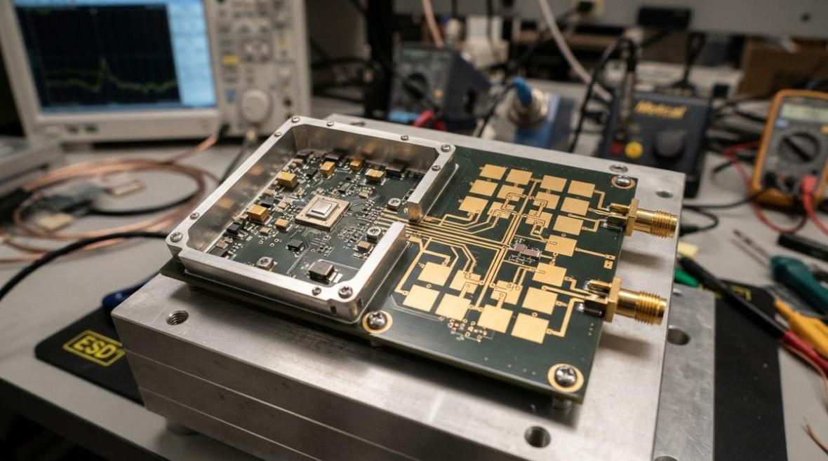
Use the tool below to set your desired scan angle, element count, and spacing. It returns the required inter-element phase shift, the steered beam pattern, and flags any grating lobes that enter visible space.

Try steering an 8-element, 0.5 λ-spaced array to 30°. You should see a main beam at 30° with no grating lobes and a beamwidth that has broadened slightly compared to broadside — roughly 14.8° instead of 12.8°. This beam broadening by a factor of approximately 1/cos(θ₀) is inherent to linear arrays. Now increase spacing to 0.7 λ and steer to 45°: a grating lobe appears near −50°, illustrating why spacing must be tightened for wide-scan arrays. If your design also needs to evaluate the complete radar detection chain, the radar link-budget calculator can convert your array gain into signal-to-noise ratio at the receiver.

From Array Factor to PCB Layout

Translating d/λ to Physical Dimensions

Once you know the required element spacing in wavelengths, convert to millimeters: d_mm = (d/λ) × (c / f), where c = 3 × 10⁸ m/s. At 24 GHz with d/λ = 0.5, the center-to-center spacing is 6.25 mm (≈ 246 mil). This spacing must accommodate the patch or slot element, the feed trace, and any ground-plane clearance — all within the tolerance budget of the PCB fabrication process.

Feed Network Considerations

A corporate (binary-split) feed network distributes power equally but consumes board area that grows with element count. A series feed is more compact but inherently frequency-squinting: the beam angle shifts with frequency because the progressive phase depends on the electrical length of each series segment. For wideband arrays, corporate feeds on low-loss laminates (Df ≤ 0.004 at the operating frequency) are preferred. When splitting power across sub-arrays, a Wilkinson divider calculator helps size the quarter-wave sections and isolation resistors.

Sidelobe Control

The −13.3 dB first sidelobes of a uniform-amplitude array are often too high for radar or communications. Applying amplitude taper — Taylor, Chebyshev, or Dolph–Chebyshev weighting — across the elements trades a slightly wider main beam for dramatically lower sidelobes. A 25 dB Taylor taper on a 16-element array broadens the beam by about 15 % but suppresses sidelobes to −25 dB, a worthwhile trade in many RCS-sensitive radar applications.

Matching and Impedance

Each element must be matched to the feed network impedance — typically 50 Ω — at the operating frequency. Mutual coupling between closely spaced elements shifts the active impedance seen by each element, sometimes by 10–20 Ω, making isolated-element S11 measurements misleading. Full-wave simulation of at least a 3 × 3 sub-array is standard practice. For impedance matching visualization, an interactive Smith chart can speed up the stub or transformer design.

Quick Design Checklist

• Set element spacing ≤ λ / (1 + |sin θ_max|) to guarantee no grating lobes over the full scan volume.
• Choose element count from the required HPBW: N ≥ 0.886 λ / (HPBW_rad × d).
• Verify with the array factor calculator above — check the steered pattern at the extreme scan angle, not just broadside.
• Apply amplitude taper if sidelobe spec is tighter than −13 dB.
• Simulate mutual coupling in a full-wave tool; adjust matching network for active impedance.
• Check PCB fabrication tolerances — at 77 GHz a ±25 µm etch tolerance on a 0.15 mm patch edge is a 17 % width error.

Frequently Asked Questions

What element spacing avoids grating lobes for all scan angles?

For a ULA that must scan to ±90°, spacing must be less than 0.5 λ. Practically, most phased arrays scan to ±60° at most, allowing spacing up to about 0.535 λ. The IEEE Transactions on Antennas and Propagation archives contain extensive treatments of this limit.

Does the array factor change with element type?

No. The array factor depends only on geometry (spacing, count) and excitation (amplitude and phase). The total pattern is the product of the array factor and the single-element pattern — so element type shapes the envelope, not the array factor itself.

How does amplitude taper affect the array factor?

Non-uniform amplitude weights lower sidelobes at the cost of a wider main beam and reduced aperture efficiency. A Chebyshev taper, for example, achieves the narrowest beam for a given sidelobe level, while a Taylor taper offers a practical compromise with controlled near-in sidelobes.

Can I use the array factor calculator for planar (2-D) arrays?

Yes. For a rectangular planar array the total array factor is the product of the linear array factors along each axis: AF_total(θ, φ) = AF_x(θ, φ) × AF_y(θ, φ). The calculators above handle the linear case; multiply two results for a separable rectangular grid.