

What a Patch Array Calculator Does
A patch array calculator takes your operating frequency, number of elements, and desired scan angle, then returns the inter-element spacing, estimated array gain, and the onset of grating lobes. For a uniform rectangular array of N × M elements on a microstrip PCB, the directivity in dBi is approximately 10·log₁₀(N·M·η) + G_element, where η is the aperture efficiency (typically 0.65–0.80) and G_element is the single-patch gain (usually 5–7 dBi). Getting the element spacing right—close enough to suppress grating lobes, far enough apart to limit mutual coupling—is the central trade-off this tool helps you resolve.
Element Spacing: The Fundamental Constraint
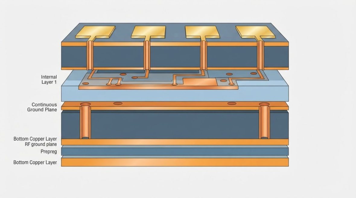
Element spacing d in a patch array is bounded by two hard limits. Too wide (d > λ₀) and grating lobes appear, stealing energy from the main beam. Too narrow (d < 0.5 λ₀) and mutual coupling degrades impedance match and distorts the embedded element pattern. The classical grating-lobe-free condition for a maximum scan angle θ_max is:
d ≤ λ₀ / (1 + sin θ_max)
At broadside (θ_max = 0°), this relaxes to d ≤ λ₀. For a ±60° scan volume the limit tightens to d ≤ 0.536 λ₀. Most practical designs target 0.5 λ₀ to 0.7 λ₀ center-to-center spacing depending on scan requirements.
Spacing Examples by Frequency
| Frequency | λ₀ (mm) | 0.5 λ₀ (mm) | 0.7 λ₀ (mm) | Typical Application |
|---|---|---|---|---|
| 2.4 GHz | 125.0 | 62.5 | 87.5 | Wi-Fi MIMO |
| 5.8 GHz | 51.7 | 25.9 | 36.2 | ISM / DSRC |
| 10 GHz | 30.0 | 15.0 | 21.0 | X-band radar |
| 24 GHz | 12.5 | 6.25 | 8.75 | Industrial radar |
| 77 GHz | 3.9 | 1.95 | 2.73 | Automotive radar |
At 77 GHz the half-wavelength spacing drops below 2 mm, which means trace-to-trace clearance on the PCB can fall under 1 mm after accounting for patch width. This puts severe demands on etch tolerance and laminate dimensional stability—one reason Rogers RO3003 laminates (Dk 3.00 ± 0.04) are widely specified for millimeter-wave arrays.
Estimating Array Gain
Array gain builds on single-element gain. For a uniform-amplitude, uniform-phase rectangular array the peak directivity is:
D_array ≈ D_element + 10·log₁₀(N_total)
where N_total = N_rows × M_columns. A 4 × 4 array (16 elements) of patches each at 6 dBi yields roughly 6 + 10·log₁₀(16) = 6 + 12 = 18 dBi before losses. Real gain is 1–3 dB lower after feed-network loss, mismatch, and scan loss are included.
To convert a gain target into an element count, or to explore how beamwidth narrows as you add rows, try the antenna gain and beamwidth calculator.
Gain vs. Element Count (Single-Patch G = 6 dBi, η = 0.7)
| Array Size | N_total | Ideal Directivity (dBi) | Typical Realized Gain (dBi) |
|---|---|---|---|
| 2 × 2 | 4 | 12.0 | 10–11 |
| 4 × 4 | 16 | 18.0 | 15–17 |
| 8 × 8 | 64 | 24.1 | 21–23 |
| 16 × 16 | 256 | 30.1 | 27–29 |
Grating Lobes and Scan Volume
A grating lobe is a full-strength replica of the main beam that appears when the path-length difference between adjacent elements equals a full wavelength. In a scanned array the grating-lobe direction θ_GL satisfies:
sin θ_GL = sin θ_scan + n·λ₀ / d, where n = ±1, ±2, …
The first grating lobe (n = −1) enters real space (|sin θ_GL| ≤ 1) when d/λ₀ > 1/(1 + |sin θ_scan|). For arrays that must steer the beam, this is the design-limiting equation. If you are designing a phased array with progressive phase shifts, the beam steering calculator lets you verify the required phase taper per element.
Voltage Spacing and Clearance on the PCB
Patch arrays often carry DC bias for active components—LNAs, phase shifters, or T/R modules—alongside the RF traces. Maintaining adequate voltage spacing between bias lines and RF ground planes is essential for reliability, especially at high altitude or in humid environments. IPC-2221B Table 6.1 specifies minimum conductor spacing as a function of peak voltage and coating condition. Enter your DC bias voltage and board parameters below to verify clearance.
For a typical 5 V bias rail on an uncoated internal layer, IPC-2221B requires a minimum spacing of 0.1 mm (4 mil). That is well within most RF PCB capabilities, but at 48 V bias (common in GaN-based arrays) the requirement jumps, and you need to plan clearance slots or conformal coating early in layout. Failing to check this can force a costly re-spin after the RF layout is locked.
Feed Network Considerations
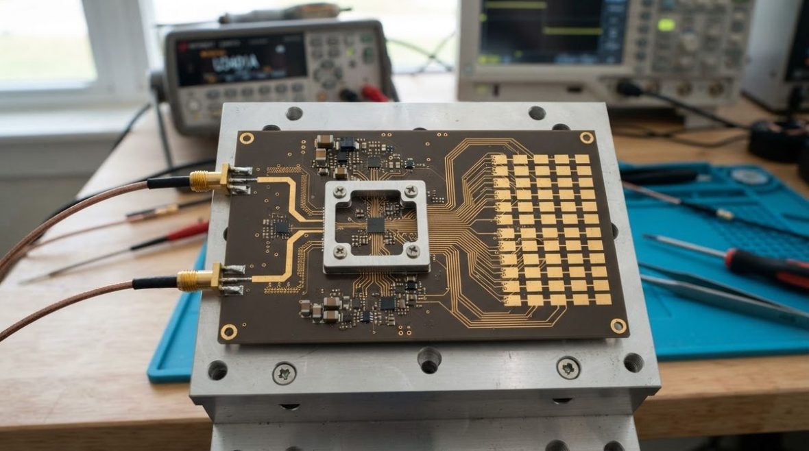
The feed network distributes power from a single input to every element. The two dominant topologies are corporate (binary tree of power dividers) and series (traveling-wave). Each has trade-offs:
- Corporate feed: Equal path lengths give uniform phase at broadside; bandwidth is limited mainly by the dividers. A 16-element corporate feed uses 15 junctions, each adding ~0.15–0.3 dB of loss on FR-4 at 5.8 GHz. On low-loss laminates like RO4350B (Df = 0.0037 at 10 GHz) that per-junction loss drops significantly.
- Series feed: Compact layout, fewer junctions, but inherently frequency-dependent beam squint. Useful for fixed-beam or narrow-band arrays.
For corporate feeds the Wilkinson divider calculator sizes each two-way split, including the quarter-wave section impedance and isolation resistor value.
Material and Stackup Selection
The substrate directly affects patch dimensions, bandwidth, and loss. Patch width W and length L scale with the effective dielectric constant ε_eff, which depends on the laminate Dk and substrate height h. A higher Dk shrinks the patch but narrows bandwidth and increases surface-wave losses. Common material choices:
| Laminate | Dk (10 GHz) | Df (10 GHz) | Best Use |
|---|---|---|---|
| FR-4 (generic) | 4.2–4.5 | 0.020 | Prototyping below 3 GHz |
| RO4350B | 3.48 | 0.0037 | 5–15 GHz arrays |
| RO3003 | 3.00 | 0.0013 | 24–77 GHz mmWave |
| RT/duroid 5880 | 2.20 | 0.0009 | Low-loss, wide-band arrays |
When your array occupies a large panel, material yield matters. A 77 GHz 12 × 12 array on RO3003 can be as small as 30 × 30 mm, but you still need to maximize the number of boards per panel to control cost. The panel utilization calculator helps estimate yield on standard Rogers panel sizes (12 × 18 in or 18 × 24 in).
Thermal Management in Active Arrays
Active electronically scanned arrays (AESAs) dissipate significant heat through T/R modules mounted directly on the PCB. At 77 GHz, SiGe or CMOS beamformer ICs may dissipate 1–3 W each, and a 256-element array can reach 200+ W total. Thermal vias under each IC are the primary conduction path to a heatsink or metal core. Use the thermal via calculator to size the via array and estimate thermal resistance from junction to board bottom.
Design Checklist for Patch Array Layout
- Set operating frequency and scan-angle requirement; compute maximum element spacing d ≤ λ₀/(1 + sin θ_max).
- Choose substrate (Dk, Df, h) and calculate single-patch dimensions (W, L).
- Determine array size (N × M) from gain target: N_total ≥ 10^((G_target − G_element)/10).
- Select feed topology (corporate or series) and simulate feed-network loss.
- Verify voltage spacing for all DC bias lines per IPC-2221B conductor spacing requirements.
- Run full-wave simulation (HFSS, CST, or openEMS) to capture mutual coupling and scan impedance.
- Check panel utilization and specify fabrication tolerances (etch ± 0.5 mil minimum for mmWave).
FAQ
What element spacing avoids grating lobes in a patch array?
Use d ≤ λ₀/(1 + sin θ_max). For broadside-only arrays, d ≤ λ₀ works; for ±60° scanning, keep d ≤ 0.536 λ₀.
How do I estimate the gain of a patch array?
Add 10·log₁₀(N_total) to the single-element gain. A 16-element array of 6 dBi patches yields about 18 dBi ideal directivity, minus 1–3 dB for feed loss and mismatch.
Can I use FR-4 for a patch array?
FR-4 is acceptable for prototyping below roughly 3 GHz. Above that, its high Df (~0.020) causes excessive feed-network loss and its Dk tolerance (±10 %) makes patch dimensions unpredictable. Use PTFE or hydrocarbon-ceramic laminates for production arrays above 3 GHz.
What is mutual coupling and how does it affect a patch array?
Mutual coupling is the electromagnetic interaction between adjacent elements. It shifts the input impedance of each element (scan impedance), distorts the embedded element pattern, and can cause scan blindness at specific angles. Coupling is strongest in the E-plane and typically ranges from −15 to −20 dB for 0.5 λ₀ spacing on standard substrates.
How many elements do I need for a 20 dBi patch array?
Assuming 6 dBi per element and 0.7 aperture efficiency, you need at least 10^((20−6)/10) ≈ 25 elements. A practical 5 × 5 or 6 × 6 array (25–36 elements) will meet this target with margin for feed loss.
Ready for a quotation?
Send your requirements for a material, stackup and manufacturing review. Price and schedule are confirmed for your project.